Gaussian graphical model node pair path statistics

Function that calculates, for a specified node pair representing endpoints, path statistics from a sparse precision matrix. The sparse precision matrix is taken to represent the conditional independence graph of a Gaussian graphical model. The contribution to the observed covariance between the specified endpoints is calculated for each (heuristically) determined path between the endpoints.

GGMpathStats(
  P0,
  node1,
  node2,
  neiExpansions = 2,
  verbose = TRUE,
  graph = TRUE,
  nrPaths = 2,
  lay = "layout_in_circle",
  coords = NULL,
  nodecol = "skyblue",
  Vsize = 15,
  Vcex = 0.6,
  VBcolor = "darkblue",
  VLcolor = "black",
  all.edges = TRUE,
  prune = TRUE,
  legend = TRUE,
  scale = 1,
  Lcex = 0.8,
  PTcex = 2,
  main = ""
)

Arguments

P0: Sparse (possibly standardized) precision matrix.
node1: A numeric specifying an endpoint. The numeric should correspond to a row/column of the precision matrix and as such represents the corresponding variable.
node2: A numeric specifying a second endpoint. The numeric should correspond to a row/column of the precision matrix and as such represents the corresponding variable.
neiExpansions: A numeric determining how many times the neighborhood around the respective endpoints should be expanded in the search for shortest paths between the node pair.
verbose: A logical indicating if a summary of the results should be printed on screen.
graph: A logical indicating if the strongest paths should be visualized with a graph.
nrPaths: A numeric indicating the number of paths (with the highest contribution to the marginal covariance between the indicated node pair) to be visualized/highlighted.
lay: A character mimicking a call to igraph layout functions. Determines the placement of vertices.
coords: A matrix containing coordinates. Alternative to the lay-argument for determining the placement of vertices.
nodecol: A character determining the color of node1 and node2.
Vsize: A numeric determining the vertex size.
Vcex: A numeric determining the size of the vertex labels.
VBcolor: A character determining the color of the vertex borders.
VLcolor: A character determining the color of the vertex labels.
all.edges: A logical indicating if edges other than those implied by the nrPaths-paths between node1 and node2 should also be visualized.
prune: A logical determining if vertices of degree 0 should be removed.
legend: A logical indicating if the graph should come with a legend.
scale: A numeric representing a scale factor for visualizing strenght of edges. It is a relative scaling factor, in the sense that the edges implied by the nrPaths-paths between node1 and node2 have edge thickness that is twice this scaling factor (so it is a scaling factor vis-a-vis the unimplied edges).
Lcex: A numeric determining the size of the legend box.
PTcex: A numeric determining the size of the exemplary lines in the legend box.
main: A character giving the main figure title.

Value

An object of class list:

pathStats: A matrix specifying the paths, their respective lengths, and their respective contributions to the marginal covariance between the endpoints.
paths: A list representing the respective paths as numeric vectors.
Identifier: A data.frame in which each numeric from paths is connected to an identifier such as a variable name.

Details

The conditional independence graph (as implied by the sparse precision matrix) is undirected. In undirected graphs origin and destination are interchangeable and are both referred to as 'endpoints' of a path. The function searches for shortest paths between the specified endpoints node1 and node2. It searches for shortest paths that visit nodes only once. The shortest paths between the provided endpoints are determined heuristically by the following procedure. The search is initiated by application of the get.all.shortest.paths-function from the igraph-package, which yields all shortest paths between the nodes. Next, the neighborhoods of the endpoints are defined (excluding the endpoints themselves). Then, the shortest paths are found between: (a) node1 and node Vs in its neighborhood; (b) node Vs in the node1-neighborhood and node Ve in the node2-neighborhood; and (c) node Ve in the node2-neighborhood and node2. These paths are glued and new shortest path candidates are obtained (preserving only novel paths). In additional iterations (specified by neiExpansions) the node1- and node2-neighborhood are expanded by including their neighbors (still excluding the endpoints) and shortest paths are again searched as described above.

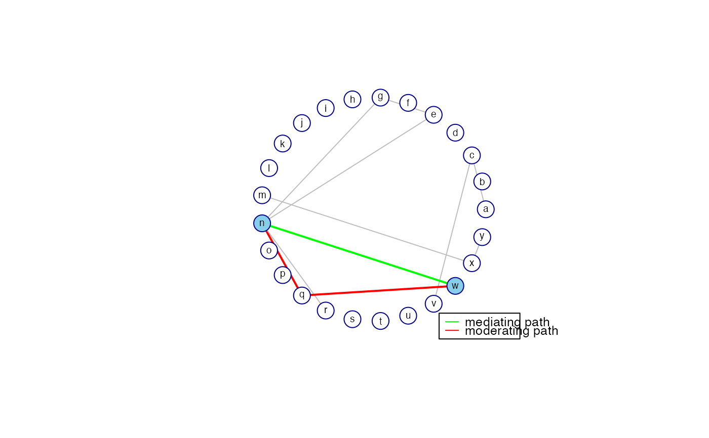
The contribution of a particular path to the observed covariance between the specified node pair is calculated in accordance with Theorem 1 of Jones and West (2005). As in Jones and West (2005), paths whose weights have an opposite sign to the marginal covariance (between endnodes of the path) are referred to as 'moderating paths' while paths whose weights have the same sign as the marginal covariance are referred to as 'mediating' paths. Such paths are visualized when graph = TRUE.

All arguments following the graph argument are only (potentially) used when graph = TRUE. When graph = TRUE the conditional independence graph is returned with the paths highlighted that have the highest contribution to the marginal covariance between the specified endpoints. The number of paths highlighted is indicated by nrPaths. The edges of mediating paths are represented in green while the edges of moderating paths are represented in red. When all.edges = TRUE the edges other than those implied by the nrPaths-paths between node1 and node2 are also visualized (in lightgrey). When all.edges = FALSE only the mediating and moderating paths implied by nrPaths are visualized.

The default layout gives a circular placement of the vertices. Most layout functions supported by igraph are supported (the function is partly a wrapper around certain igraph functions). The igraph layouts can be invoked by a character that mimicks a call to a igraph layout functions in the lay argument. When using lay = NULL one can specify the placement of vertices with the coords argument. The row dimension of this matrix should equal the number of (pruned) vertices. The column dimension then should equal 2 (for 2D layouts) or 3 (for 3D layouts). The coords argument can also be viewed as a convenience argument as it enables one, e.g., to layout a graph according to the coordinates of a previous call to Ugraph. If both the the lay and the coords arguments are not NULL, the lay argument takes precedence

The arguments Lcex and PTcex are only used when legend = TRUE. If prune = TRUE the vertices of degree 0 (vertices not implicated by any edge) are removed. For the colors supported by the arguments nodecol, Vcolor, and VBcolor, see https://www.nceas.ucsb.edu/sites/default/files/2020-04/colorPaletteCheatsheet.pdf.

Note

Eppstein (1998) describes a more sophisticated algorithm for finding the top k shortest paths in a graph.

References

Eppstein, D. (1998). Finding the k Shortest Paths. SIAM Journal on computing 28: 652-673.

Jones, B., and West, M. (2005). Covariance Decomposition in Undirected Gaussian Graphical Models. Biometrika 92: 779-786.

Author

Wessel N. van Wieringen, Carel F.W. Peeters <carel.peeters@wur.nl>

Examples


## Obtain some (high-dimensional) data
p <- 25
n <- 10
set.seed(333)
X <- matrix(rnorm(n*p), nrow = n, ncol = p)
colnames(X) <- letters[1:p]

## Obtain regularized precision under optimal penalty
OPT <- optPenalty.LOOCVauto(X, lambdaMin = .5, lambdaMax = 30)

## Determine support regularized standardized precision under optimal penalty
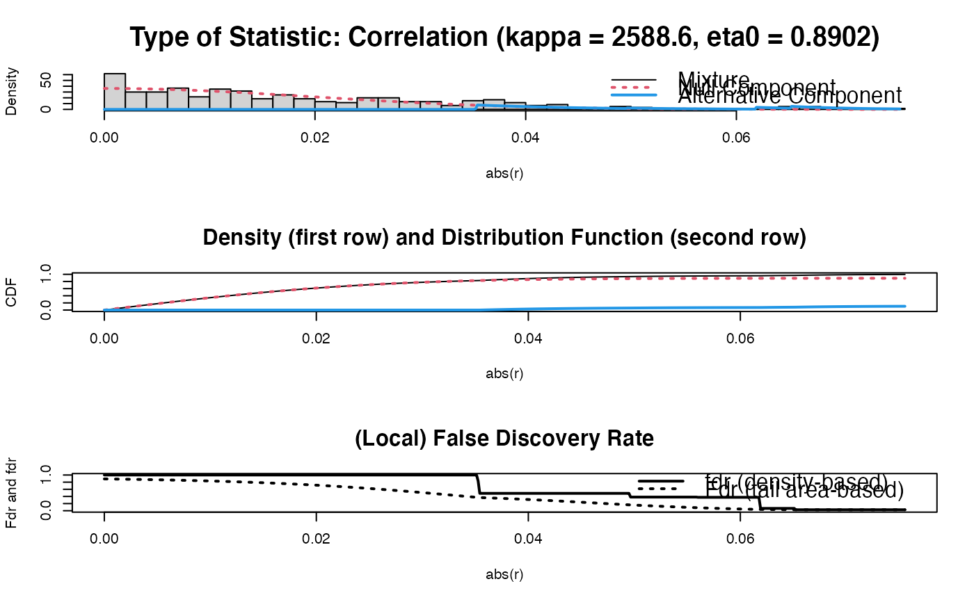
PC0 <- sparsify(OPT$optPrec, threshold = "localFDR")$sparseParCor
#> Step 1... determine cutoff point
#> Step 2... estimate parameters of null distribution and eta0
#> Step 3... compute p-values and estimate empirical PDF/CDF
#> Step 4... compute q-values and local fdr
#> Step 5... prepare for plotting

#> 
#> - Retained elements:  11 
#> - Corresponding to 3.67 % of possible edges 
#>  

## Obtain information on mediating and moderating paths between nodes 14 and 23
pathStats <- GGMpathStats(PC0, 14, 23, verbose = TRUE, prune = FALSE)
#> Covariance between node pair : 0.06757 
#> ----------------------------------------
#>         path length contribution
#> 1     14--23      1      0.07211
#> 2 14--17--23      2     -0.00453
#> ----------------------------------------
#> Sum path contributions       : 0.06757 
#> Warning: 'as.is' should be specified by the caller; using TRUE
#> Warning: 'as.is' should be specified by the caller; using TRUE

pathStats
#> $pathStats
#>            length contribution
#> 14--23          1  0.072107158
#> 14--17--23      2 -0.004533758
#> 
#> $paths
#> $paths$`14--23`
#> + 2/25 vertices, named, from f65fc2a:
#> [1] 14 23
#> 
#> $paths$`14--17--23`
#> + 3/25 vertices, named, from f65fc2a:
#> [1] 14 17 23
#> 
#> 
#> $Identifier
#>    Numeric VarName
#> 1        1       a
#> 2        2       b
#> 3        3       c
#> 4        4       d
#> 5        5       e
#> 6        6       f
#> 7        7       g
#> 8        8       h
#> 9        9       i
#> 10      10       j
#> 11      11       k
#> 12      12       l
#> 13      13       m
#> 14      14       n
#> 15      15       o
#> 16      16       p
#> 17      17       q
#> 18      18       r
#> 19      19       s
#> 20      20       t
#> 21      21       u
#> 22      22       v
#> 23      23       w
#> 24      24       x
#> 25      25       y
#>